ImageSurfer Tutorial: Volume Rendering Dendritic Spines
ImageSurfer is a tool that visualizes 3D data. This tutorial describes how to use ImageSurfer to generate Direct Volume Renderings (DVRs).
Loading Data

- Enabling volume rendering in ImageSurfer
The first step is to get your data loaded into ImageSurfer. The tutorial on isosurfaces describes this procedure in more detail, so follow the steps there. Once the data is loaded, you must enable volume rendering by choosing Volume Render from the Render Style from the Dataset tab of the ImageSurfer window. The figure to the left shows where this box is located in the ImageSurfer interface. Be sure to click the Apply Changes button after selecting the new render style.
DVR is a technique for drawing 3D data sets that composites all of the data voxels onto the screen. Of course, data values by themselves cannot be superimposed on the screen, so a transfer function is necessary to map data values into colors and opacities. The bottom of the ImageSurfer window contains a transfer function editor.

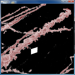
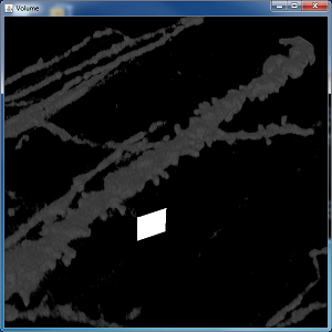
- Volume rendering of the dendritic spine data with default settings.
This tutorial will demonstrate DVR for the dendritic spine data set also used for the isosurface tutorial. After enabling DVR, the volume window should update and contain a DVR that uses a default transfer function to project the 3D data set into an image. The figure on the left shows what this looks like for the dendritic spine data. By default, this image is not tremendously useful; the spine is visible in white, but is surrounded by a sea of red that occludes everything within. To improve this function, we first need to understand what a transfer function is and how to modify it.
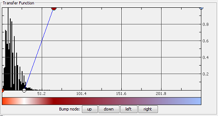
The figure below is a zoomed up transfer function editor. The horizontal axis of the chart is the range of the data values in the data set. ImageSurfer automatically calculates the minimum and maximum values and clamps them to the left and right respectively. For example, an 8-bit image that can potentially range from 0 to 255 may actually only contain values in the range 50 to 150. The black bar chart in the background of the plot is a histogram of the data. In this example we can see that most of the values in the dendritic spine data set are between 0 and 50, although a few do appear in the high ranges. The vertical axis of the plot is opacity, so the transfer function, drawn as a blue segmented line, describes how any data value on the horizontal axis maps to opacity in the vertical axis.
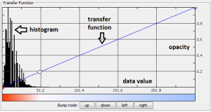
- A closer look at the transfer function editor.
Additionally, there is a color scale at the bottom of the editor. This describes how a data value is mapped to a color value. Now we can understand the white dendrite floating in a sea of red. The low values are all red or pink with low opacity. The mid-range values are all white with medium opacity. The high range values are all blue, with high opacity. However, because there are only very few high range values, no blue appears in the rendering.

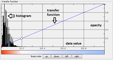
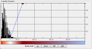
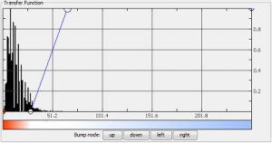
- Modifying the transfer function to clear out low values.
You can control the shape of the transfer function by moving, inserting, or deleting nodes (the circles) from the plot. To move a node, left-click and drag it to the desired position. For our example data set, we know that the dendrite is already highlighted reasonable well in white, but the sea of red is uninteresting. After being moved down to the bottom of the plot, the segment connecting the red node to the white node now has no opacity in the image. The result is that the lower values will not appear.
- Volume rendering with the new transfer function. The red background is gone.

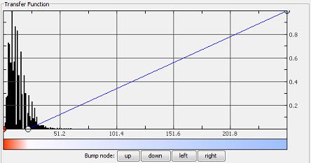
The volume window now shows more-or-less what we expected to see. The red background is gone, leaving a white dendrite floating in space. This image demonstrates one of the problems that occur when using DVR. The image is blurry, lacking important details of the shape of the dendrite. We can ameliorate this a bit by improving the transfer function. The first problem is that opacities ramp linearly from 0 to 1 between the white and blue nodes. This means that the majority of the dendrite voxels are mostly transparent, which makes the image very blurry. We therefore need to modify the transfer function so that the range of values of the dendrite are more opaque. The solution is to add a new node in the transfer function that has a higher opacity.
- Adding a sharp jump in opacity.
We can add the new node by right-clicking on the line where we want to add a new node and choosing Insert color node from the context menu. A new node will appear with a default black color. We can make the dendrite voxels more opaque by dragging the new node up to the top of the editor. To differentiate them from the background better, we can give the node a different color by right-clicking on the node and selecting Choose color from the context menu. A window containing a wide array of colors will appear. In this case, we’ve chosen a maroon color.
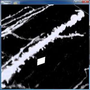
- Volume rendering with a large jump in opacity highlights surfaces.
Look at the resulting image on the left. The inside of the dendrite is now maroon and the outside of the dendrite is white. This means that the voxels within the dendrite have higher values that the voxels outside the dendrite. Using color to differentiate the inside from the outside of the dendrite is a useful way to see surface details, including the shapes of the small spines growing off of the dendrite.
Notice that the image is much clearer. This is because there are much fewer transparent voxels. In fact, if we move the opaque maroon node all the way to the left so that the transfer function is a step function, the image will closely resemble an isosurface without any surface shading. The glowing effect is useful in this respect, as it gives hints about the shape of the surface. Proper surface shading can be done with a separate technique called Directionally-Illuminated Direct Volume Rendering (DIDVR). First we will change the maroon node to white, for reasons that will become clearly shortly.
- Setting the dark red node to white.

- Directionally illuminated volume rendering shows surface shape, but is much dimmer.
We will also need to change the render style to Directionally Illuminated Volume Rendering in the same drop down box as before. Again, be sure to click Apply Changes. The resulting image appears to the right. DIDVR removes brightness to emphasize regions of the data set that have high gradient. This is the reason that the image is so dim. However, if you look closely you will see that it is possible to see the shape of the spine, albeit dimly.