Network Extractor Tutorial

This tutorial shows you how to use the Network Extractor program to calculate fiber segment orientation histograms from 3D images of fibrous objects.

Preparation

Network Extractor has been designed to operate on images of fibrous objects where the objects are brighter than the background intensity. Widefield and confocal fluorescence microscopes produces such images.

Starting the program

On Mac OS X, open a Finder window and navigate to the Applications directory. Double-click the NetworkExtractor 1.0.0 program.

On Windows XP, click the Start menu and select All Programs->NetworkExtractor 1.0.0->NetworkExtractor 1.0.0.

Loading the image

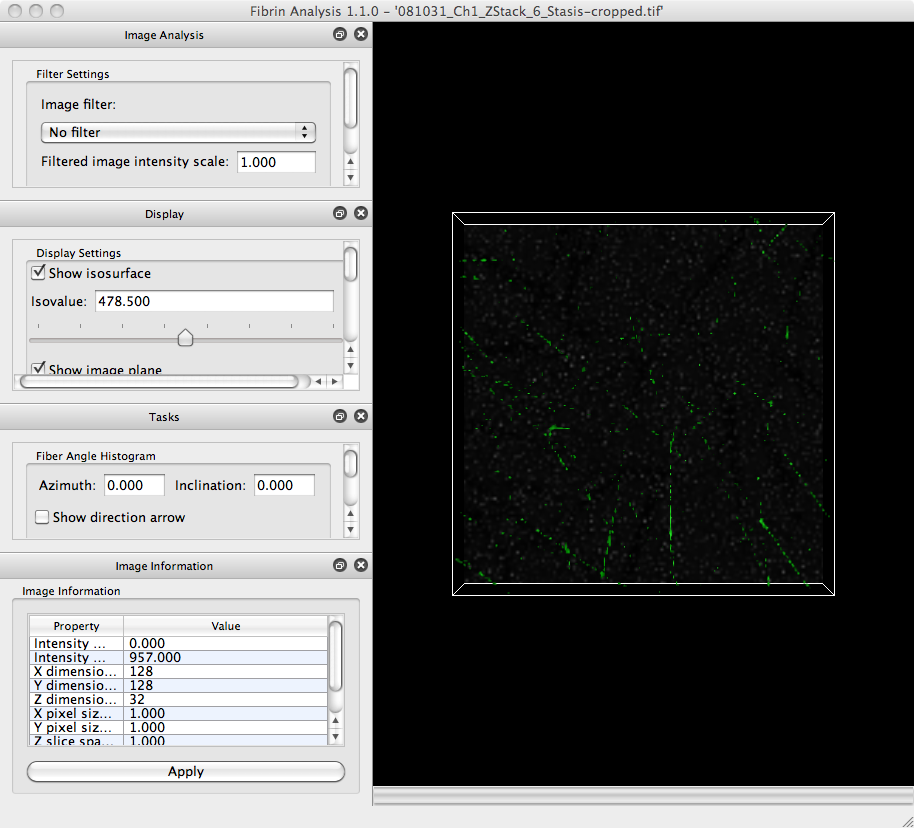
Download the image for this tutorial (generously provided by Alisa Wolberg’s laboratory)) and save it to your hard drive. In NetworkExtractor, click on the File menu and select the Open Image. item. In the file browser that appears, navigate to the location where you saved the tutorial image. The program may take a moment to load the image. Once it is loaded, the program window should look like:

Network Extractor after loading an image. — Network Extractor after loading the tutorial image.

View image slices

The large portion of the window with the black background is called the Visualization Panel. It displays two visualizations of the image you just loaded.

Slice plane

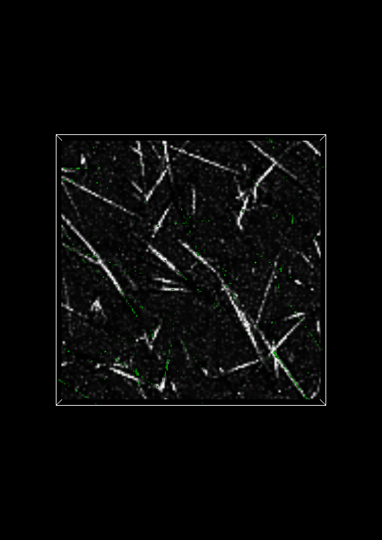
A slice plane shows a single z-slice from the 3D image. It is initialized to the bottom-most slice in the stack (z=1). To change which slice is displayed, find the Display control panel and look for the Z plane control. The text box shows which slice is displayed. You may change this slice by typing the slice number in the text box or by sliding the horizontal slider control just underneath the Z plane control.

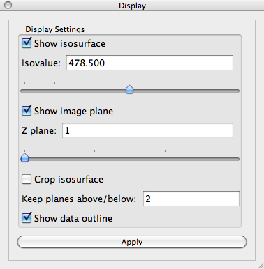
Change the image Z plane to 11. The Visualization Panel should now look like:

Results of moving the image plane to the 11th slice.

Isosurface

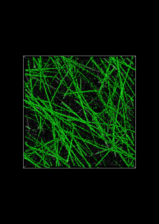
An isosurface is a surface that represents a boundary between two parts of an image. One part of the image is defined as the regions where the intensity is greater than or equal to a specified isovalue. The other part of the image are all the regions not in the other part, that is, where the intensity is lower than the specified isovalue. In effect, the isovalue is a threshold that separates the two parts of the image, and the isosurface displays where this separation occurs.

In the Display window, change the Isovalue: to 100 and click on the Apply button at the bottom of the Display control panel. The Visualization Panel should now look like:

The isosurface generated at isovalue 100.

Changing Image Settings

To perform quantitative image analysis, it is important that the physical dimensions of the image are specified correctly. This includes specifying the pixel size and slice spacing, both in microns, in the last few rows of the table in the Image Information window. For this image, the pixel size is 450 nm and the slice spacing is 1 µm. Change the settings so that they match those in the image below:

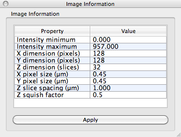
Image Information window with settings for the loaded image.

Notice the Z squish factor setting at the bottom of the table. In confocal microscopy, objects are elongated in the z-direction because of the point-spread function. Fibrous objects, therefore, appear not as tubes, but as tubes fattened up in the z-direction. The z-squish factor is meant to counter this extension in z. It specifies a scaling factor that should applied in only the z-direction. After the scaling is applied, the fibrous objects appear more tubular. Setting the Z squish factor to 1.0 preserves the original z-spacing in the image. For this data set, a Z squish factor of 0.5 works well because z-resolution in confocal images is roughly half the resolution in the x– and y-directions. Note: all orientations we will calculate later in the tutorial will correct for this Z squish factor.

Click the Apply button to update the image.

Computing Fiberness

In general, fluorescence images of fibrous networks cannot be adequately segmented by intensity values alone. This is especially true in the case of images taken with nonuniform lighting conditions or containing both thick (bright) and thin (darker) fibers.

Instead of using intensity threshold, Network Extractor computes what is called a fiberness measure. Fiberness is derived from looking at second-derivative information in the image. Intuitively, for fibrous objects, the second derivative along the fiber axis does not change much, while second derivatives in any direction orthogonal to the fiber axis do change. The algorithm used to compute fiberness operates at multiple scales, meaning it can identify fibers of differing radii.

In the Image Analysis control panel, change the Image filter setting to Multiscale Fiberness. The fiberness filter is controlled by several settings shown here:

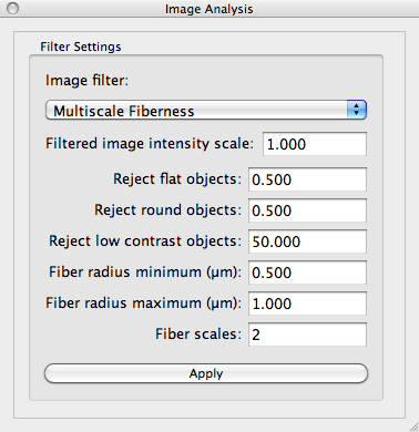
Image Analysis window with settings for the Multiscale Fiberness filter.

Enter the setting values shown and click the Apply button. The settings are explained below:

Reject flat objects – Weighting factor that controls how the filter differentiates fibrous objects from thin, flat objects. Higher values tend to reject flat objects. Setting this value to 0.5 typically works well.
Reject round objects – Weighting factor that controls how selective the fiberness filter is for fibrous objects versus sphere-like objects. Lower values tend to reject sphere-like objects. Setting this value to 0.5 typically works well.
Reject low contrast objects – Weighting factor that controls the how much brighter than background objects must be to be identified as fibrous. Higher values of this setting identify highly contrasting fibrous objects. This setting can be important to reduce occurrences of background noise being misidentified as a fibrous object. A value of 50.0 often works well for microscopy images.
Fiber radius minimum (μm) – The minimum radius of fibrous objects to be identified by the filter specified in microns.
Fiber radius maximum (µm) – The maximum radius of fibrous objects to be identified by the filter specified in microns.
Fiber scales – The number of scales, including the minimum and maximum scales, that will be used to identify fibrous objects. This must be at least 2. The scale space is examined at scale i*(fiber radius maximum – fiber radius minimum)/(fiber scales-1)where i is the ith scale.

Evaluate the Fiberness Computation Results

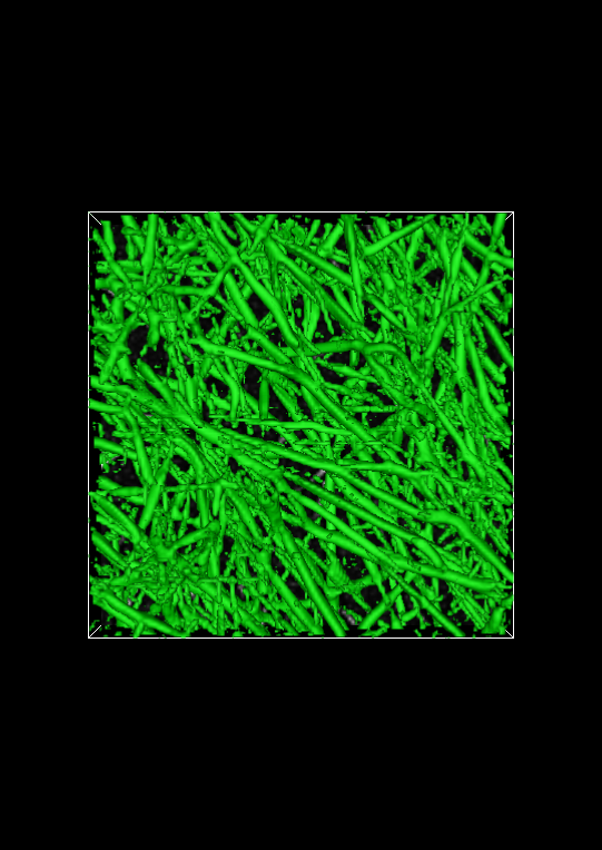
The isosurface visualization method can be used to evaluate how well the multiscale fiberness filter identifies fibers. Before evaluation of the filter can take place, a suitable isovalue must be found. This can be done by changing the isovalue slider in the Display window. If the isovalue is too high, individual fibers will appear to be broken into multiple fibers. If the isovalue is too low, noise that does not correspond to an actual fiber may appear in the isosurface.

The image below shows the full isosurface at isovalue 0.25. This isovalue segments the fibrous objects in the image quite well. Set the isovalue to 0.25, and click the Apply button.

Isosurface of fiberness filter result (isovalue = 0.25).

Spot check the segmentation

Evaluating the fiberness-based segmentation is not usually possible by looking at the entire isosurface. Fortunately, Network Extractor has a visualization mode that enables you to look at thin slabs of the isosurface at a time. Basically, this means that the isosurface is cropped above and below some reference plane. In Network Extractor, the reference plane is the image plane. When the Crop isosurface checkbox is checked, only a thin section of the isosurface in the z-direction will be visible above and below the image plane. An example of what this looks like is shown below.

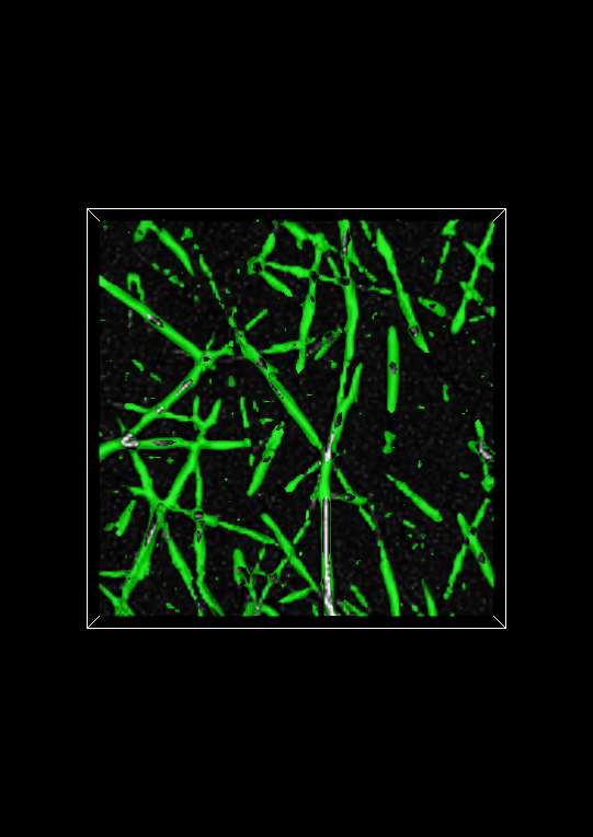
Cropped isosurface visualization for evaluating segmentation results (keep planes above/below = 5).

To evaluate the segmentation, you can compare the cropped isosurface to the image. The isosurface is green and the image is grayscale. Evaluation, roughly speaking, is therefore ensuring that where there is white in the image, there is also green. You can adjust the number of planes above and below the image (the Keep planes above/below option) plane to get a good tradeoff between defining the isosurface sufficiently and seeing the image plane clearly. If you use too few planes, the isosurface will look like a very thin contour line on either side of a fiber in the image plane widget, assuming the multiscale fiberness segmentation worked well.

Set the value of Keep planes above/below to 5 and click Apply. In this example, the isovalue appears to give a good segmentation of the fibers in the image. If it did not, you would want to do two things:

Change the isovalue to find a better match between the isosurface and the image.
Change the multiscale fiberness filter settings.

Skeletonization

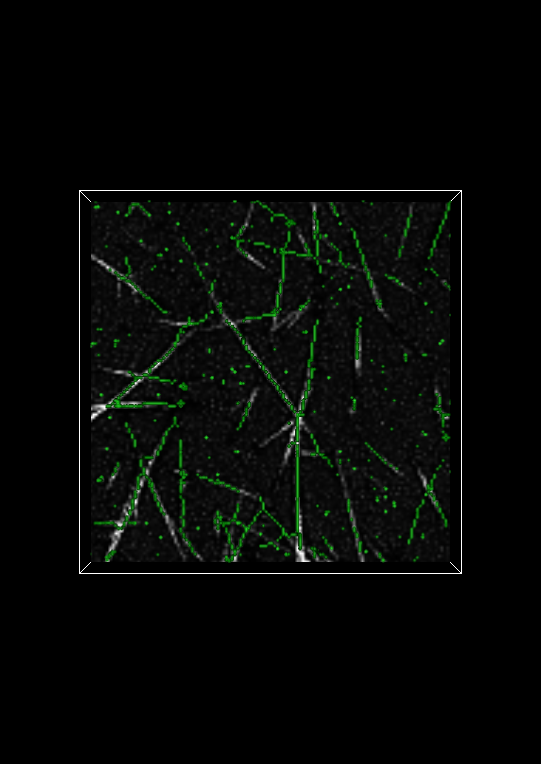
Now that we have found a good isovalue that segments the fibers, we can proceed to compute orientation statistics on the fibers. We want to compute fibrin orientation statistics on short segments of fiber rather than over individual fibers. Moreover, we want the statistics to be insensitive to fiber width. One way to meet both requirements is to locate voxels near the centers of fibers. This is the so-called skeleton of the fibers, and finding it is called skeletonization.

Broadly speaking, the voxel size is the size of one fiber segment. To avoid bias based on fiber orientation, the image is resampled to have cubic voxels. If this resampling were not performed, then fibers oriented along the z-direction would typically be counted fewer times because z-slice spacing is typically larger than the pixel size in fluorescence microscopy images.

To compute the skeleton select the Skeletonization filter in the Image Analysis window. You may notice that a new setting called Fiberness Threshold appears. Set this value to the isovalue we determined above: 0.25. Click Apply. The Display Panel will now appear like below:

Results of skeletonization at fiberness threshold 0.25.

Saving Orientation Statistics

During the fiberness computation, the orientation of the fiber passing through each voxel is computed. Network Extractor lets you save this orientation information in one of two ways.

The first way is to save the raw orientation information at each skeleton voxel along with the coordinates of the voxels. To save this information, select the Save Fiber Orientation Data… in the File menu. The output is a CSV spreadsheet file containing six columns:

xPosition – The x-coordinate of the fiber voxel.
yPosition – The y-coordinate of the fiber voxel.
zPosition – The z-coordinate of the fiber voxel.
xDirection – The x-component of the fiber orientation vector.
yDirection – The y-component of the fiber orientation vector.
zDirection – The z-component of the fiber orientation vector.

Save the fiber orientation data to a file called ‘orientation-data-raw.csv’. You can then process this spreadsheet data in your favorite statistical analysis software package.

The second way is to save an orientation histogram computed by the program. The histogram is of angles formed between a reference direction and the orientation of voxel-sized segments along fibers. Orientations of fiber segments are specified by 3D vectors. All orientation vectors are processed so that they point in a set of directions defining a hemisphere. The hemisphere is defined by the plane orthogonal to the reference direction. The re-orientation process ensures that angles between a fiber segment and the reference direction are in the range [0, 90] degrees. To set the reference direction, you can change the Azimuth and Inclination parameters. We’ll leave the default values for these settings which defines a direction pointing in the positive x-direction. We’ll also use the default number of bins in the histogram.

Save the orientation histogram by clicking the Save angle histogram button in the Tasks window. Name this file ‘orientation-data-histogram.csv’. The file consists of five columns:

Angle (deg.) – The minimum value in the histogram bin. The maximum value in the histogram bin is given by the next row in this column. The maximum angle on the last bin is 90 degrees.
Count – The number of image voxels in the histogram bin.
Normalized Count – The number of image voxels in the histogram bin divided by the total number of voxel values in the histogram.
Expected Probability – The expected normalized histogram value for an object with uniform randomly distributed orientation of fiber segments.
Over-representation Ratio – The normalized count divided by the expected probability. This gives an indication of whether and to what degree the orientations within a histogram bin are overrepresented. A value of 1.0 means the number of orientations of fiber segments falling into this bin is expected, a value below 1.0 means there are fewer fiber segments falling in this bin than expected, and a value above 1.0 means there are more fiber segments falling into the bin than expected for an object with uniform randomly distributed orientations.

Congratulations!

You have completed the Network Extractor tutorial and are now ready to try the program on your data.