This tutorial shows you how to use ImageSurfer2 to generate the skeleton of the fibers in the microscopy fibrin image and then label the branch points of this skeleton.

Preprocess Step for Z Blurring Image:

The filters we are using rely on the structures we seek being tube-like in 3D, so preprocess is needed for datasets that have blurring in Z which makes them slab-like (tall and skinny). Probably the best solution to this will be to run deconvolution filter which should be ready soon. However, currently we provide a sample matlab file which can do resampling to reduce the tubes back to being round (See Appendix). Make sure you set the z spacing the same as the original one so that the resample does influence.

Basic computing steps:

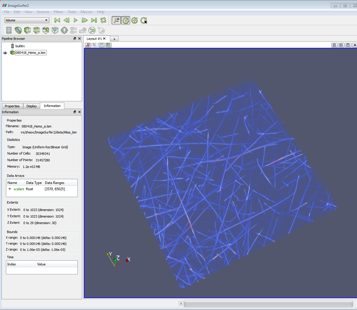
1. Load the .lsm image. See http://cismm.web.unc.edu/resources/tutorials/imagesurfer-2-tutorials/
for instruction of loading data and volume rendering for the 3D images. After
loading the image, some useful information about the image can be found on the
information tab. (e.g. Data ranges, Extends, Bounds)

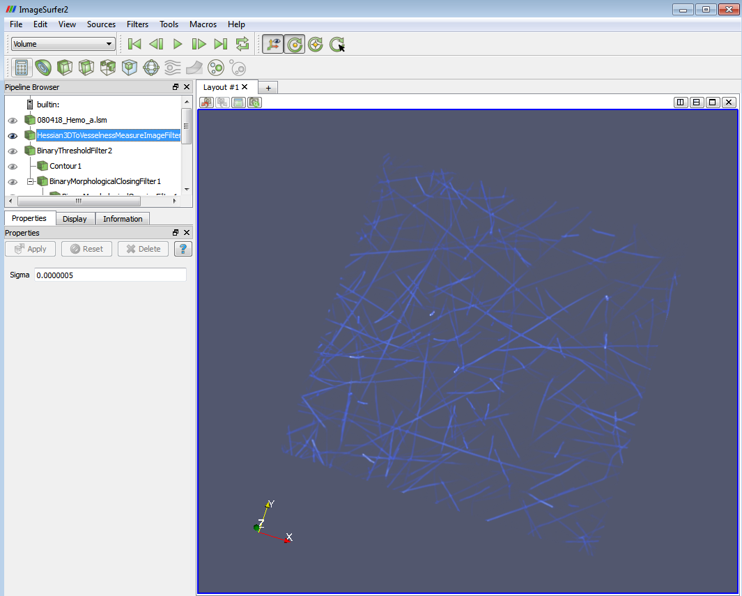
2. Apply the “Hessian 3D to vesselness measure image filter”. You can find all the “filters” from the main menu->filters.

This is a line filter to provide a vesselness measure for tubular objects from the hessian matrix and is used to discriminate the bright tubular structures. Notice the parameter “Sigma” is in physical space unit. So you will need to check the image spacing when you set it. I use 0.0000005 (0.0005 for ImageSurfer 2.4.4) to the image which has spacing of

0.000146, 0.000146, 1.06e-5 in x,y,z direction. (In ImageSurfer 2.4.4, the numbers are 0.146, 0.146, 0.0106)

Sigma is the physical width of the desired tubes. To get a good estimate of an appropriate Sigma, you first need to compute physical distance/pixel. For example in this case, the x width of this example is 0.000146 (nm) over 1024 pixels, so nm/pixel is 0.000146/1024=0.00000014. To extract tubes of 5 pixels wide, we specify 0.00000014*5=0.0000007 (nm) in the Sigma.

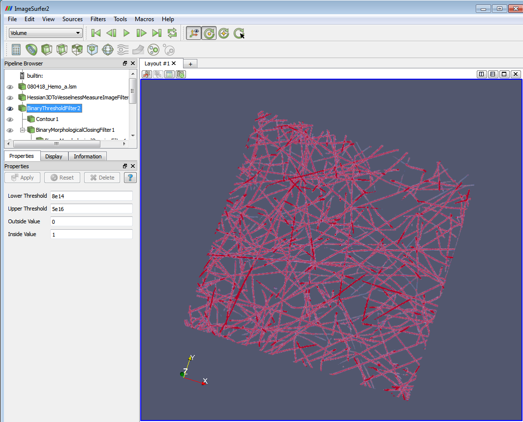
3. Apply the “Binary Threshold filter”. Set the ‘Lower Threshold’ to 0 and ‘Upper Threshold’ to 5e14.  5e14 is roughly below the maximum pixel value (5.5e+16) in the dataset, which can be obtained from the Information tab after applying the Hessian filter.  Set the ‘Outside Value’ to 1 and ‘Inside Value’ to 0. If the result doesn’t show clearly, click “rescale to image” in the display tab.

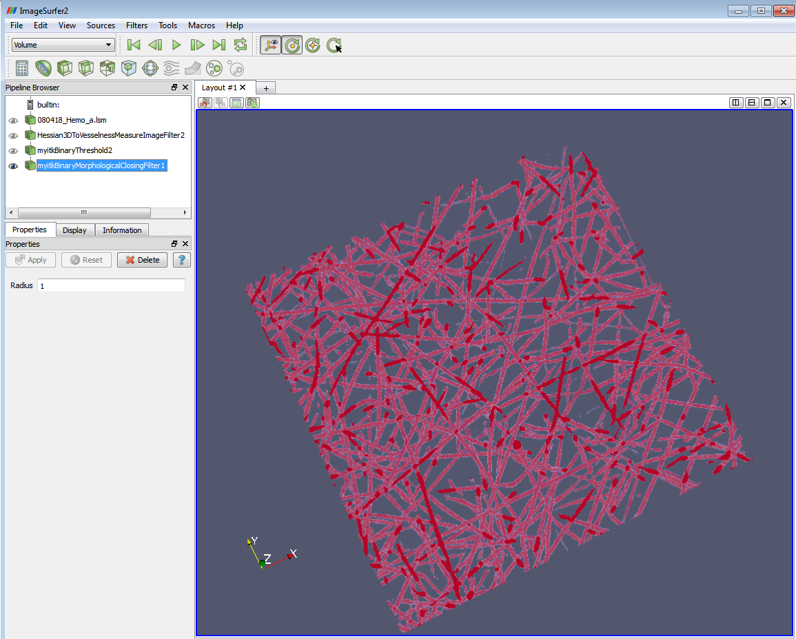
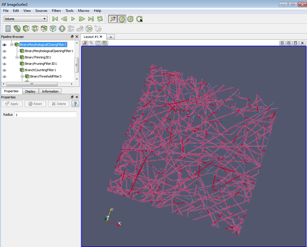
4. Apply the “Binary Morphological Closing Filter”. This filter removes small (i.e., smaller than the structuring element) holes and tube like structures in the interior of the image. The morphological opening of an image “f” is defined as: Closing(f) = Erosion (Dilatation (f)).

5.There are also 3 other morphological image filters implemented which are the “Morphological opening image filter”, “Binary erode image filter” and the “Binary dilate image filter”. They are used to filter out “positive” detail of the image, shrink the image and expand the image respectively. You can choose different combination of these morphological image filters to find out which works best.

The parameter “Radius” means the radius of the structuring element used in the morphological process. The default value is 1 voxel. Then the structure element would be a 3-by-3 ball. You might need use larger “Radius” for the closing image filter to avoid the blob-like structure (arrow). They are due to the cavities in the original object which are preserved and eroded from the inside by the algorithm. This blob-like structure will lead to the major outliers in branch-counting step, i.e. label points by the number of fiber branches there.

The result of the morphological filters would be like the following:

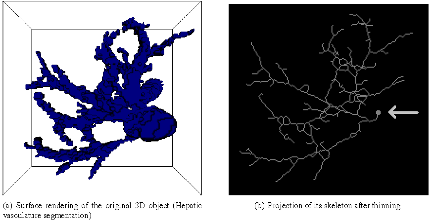
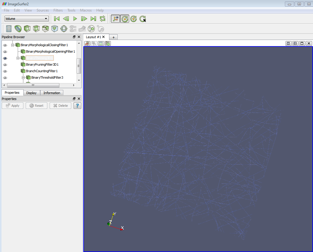
6. Apply the “Binary Thinning 3D” filter.  This filter generates the 1-voxel-wide centerline of the binary image and preserves the topology and geometry characters during the process.

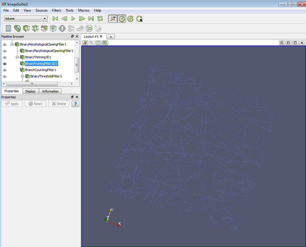
7. Apply the “Binary Pruning Filter 3D” filter. Branches that are less than a certain length are pruned. It is set to 3 by default currently.

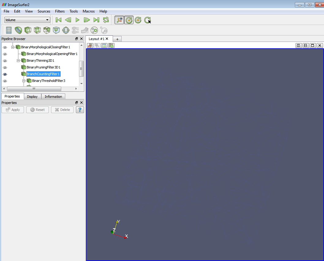
8. Apply the “Branch counting filter”.

This filter is used to count branch numbers for every point in pruning result image. The ones labeled “2” are in the middle of a fiber and are related to total fiber length.  The ones labeled “3”+ indicate branch points in common sense, and are related to the connectivity.  The ones labeled “1” are at the ends of fibers. And “0” means background points. So the result of this filter is a scalar field.

As the 1-branch points on the boundary are most probably not the actual end points, we label them as regular (2-branch) points. As the thinning process might somehow shorten the fiber for a little, “Boundary” here is not considered just as the most outside layer of the image but as of some thickness. The “HandleBoundaryRadius” parameter gives the thickness of the boundary.

The “BranchCombineRadius” parameter gives the distance of two 3-branch points below which they are “combined” as a 4-branch point. Read the fifth term in “Brief Method Description” section for details.

In this example, after the branch counting filter, the Data Ranges shown on the information tab are [0, 6]. These numbers are too small for the scalar field to be shown clearly. Next section will show you how to highlight each type of branch points separately on the original or the skeleton image.

Visualization and Analysis of the results:

To highlight the branch points using contours, please follow a) in the 3^rd and 7^th steps. To highlight them using glyphs, follow b) in these two steps.

1. Apply “Binary threshold filter“ on the branch counting resultant scalar field. This enables us to show one specific type of branch points each time. For example, set the ‘Lower Threshold’ and ‘Upper Threshold’ to 3 and 4 to display 3-way and 4-way branches. Set them both to 3 to display only 3-way branches.
2. Apply “Contour” filter (“Value” set to 0.5) on the resultant binary image.
3. a) Change representation from “Surface” to “Points” in drop-down list on top. Switch to the Display tab and click “Set Solid Color”. Then you can choose a color for your isosurface. b ) Apply “Glyph” filter to the contour. Set “Glyph Type” to “sphere”. Set proper sphere “Radius” (maybe 0.1-0.5). Turn off “Mask Points” check box. (You can change colors for skeleton/ sphere/background if you want).
4. In the Pipeline Browser, select the thinning resultant binary image or the original grayscale .lsm image.
5. Change representation type to “Volume”.
6. If it doesn’t show clearly, click “rescale to image” in the display tab.
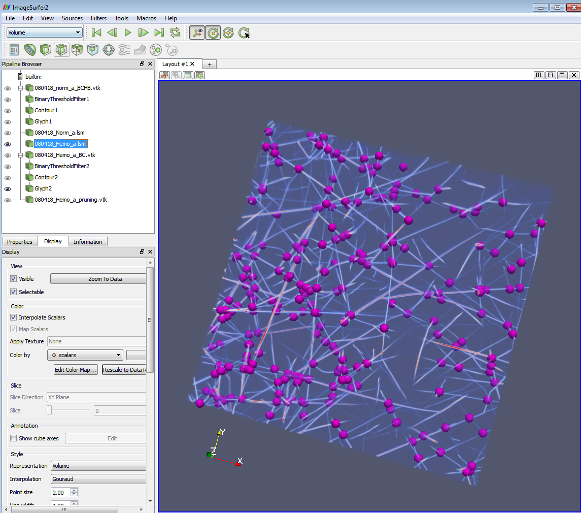
7. a) Now you can see the branch points and the image at the same time. E.g. if the threshold you set in (1) is 2.5-3.5, you will see an image with all the 3-branch points highlighted on it. The following two images show 4-branch points with skeleton and with volume rendering.

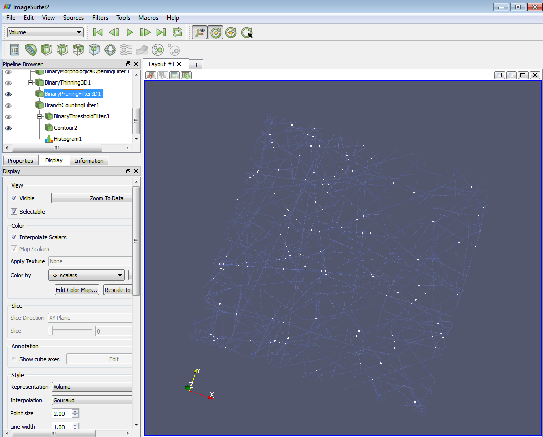
4-branch points highlighted on the skeleton image

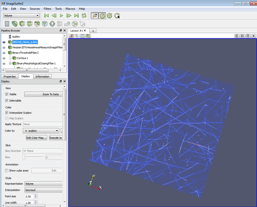
4-branch points highlighted on the original lsm image.

b) Wear 3D glasses. Set proper 3D properties for the monitor: 3D mode/ LR change… Then you can see the branch points (shown as glyphs) and the image at the same time. E.g. if the threshold you set in (1) is 2.5-3.5, you will see an image with all the 3-branch points highlighted on it.

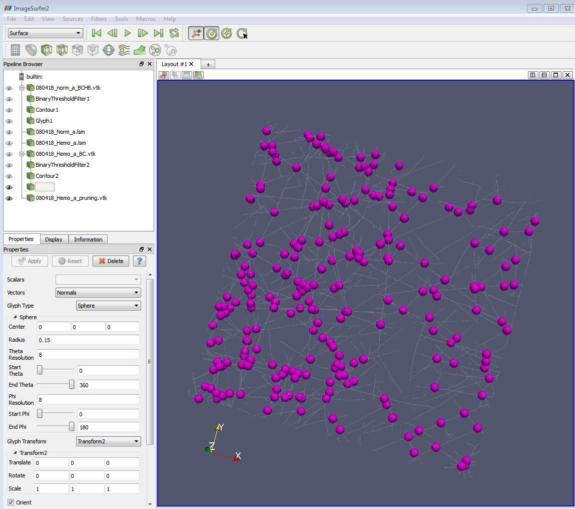
4-branch points highlighted (drawing glyphs) on the skeleton image

4-branch points highlighted (drawing glyphs) on the original lsm image

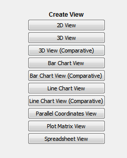
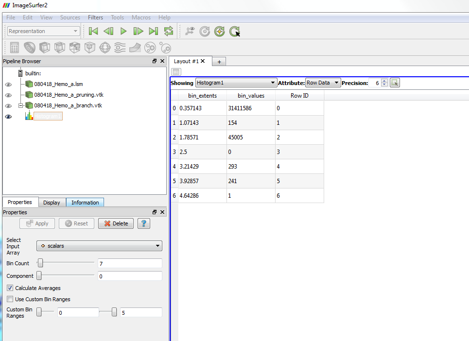
8. To get the exact numbers of the branch points, you can apply “Histogram” filter to branch counting resultant image. Set “Bin Count” to the number of branch types. Create a Spreadsheet View to view the result by first create a new layout

And then click the “Spreadsheet View” button on the bottom.

You will have the numbers of all types of “branch” points (including the 0-branch background points, 1-branch end points and the 2-branch regular points). You can also save the spreadsheet as a .cvs file which can be open using other software.

9.To get the positions of some kind of branch points. After you get the binary image in the first step, apply “Image Data to Point Set” filter.

Then apply the “Mask Points” filter. Set “On Ratio” to 1, “Maximum  Number of Points” to a pretty large number, like 999999999 (that means we don’t want any point to be discarded), and have the “Generate Vertices” and “Single Vertex Per Cell” boxes checked.

Then apply the “Threshold” filter. Set “Lower Threshold” and “Upper Threshold” to 0.5 and 1.5 respectively.

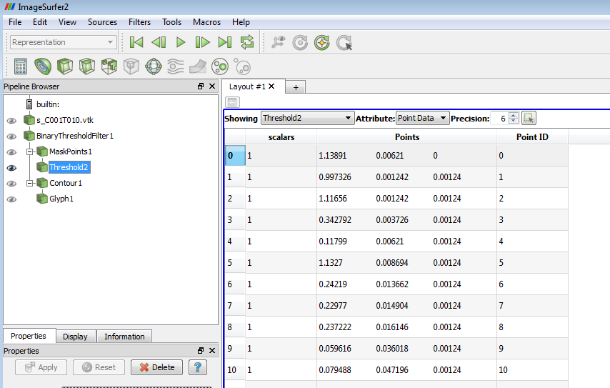
Now you can view the result in a “Spreadsheet View” (refer the 8th step for how to create a spreadsheet view) or save it as a “.csv” file. The first column represents the scalar values (all are “1” in our case because we have segmented the foreground points using threshold filter). The following three columns represent the physical coordinates of the points.

Reference:

Appendix:

To create a sub-stack, you can use Fiji (ImageJ), Image > Stacks > Tool > Deinterleave, and use every N slice you’d like to extract as the number of channels in deinterleave, e.g. deinterleave a stack into 5 channels would produce a stack containing slices of 1, 6, 10, 15…

% This is a sample matlab file which resamples images in z direction (1: 5).% It just handles tiff images. for i = 1:136  % num of files in the time series    for j = 1:32  % numOfStacksInZ / 5        oldfilename = Strcat(‘.\origin\’, ‘s_C001’,…       ‘T’,num2str(i,’%03d’),’Z’,num2str(j*5,’%03d’),’.tif’);        newfilename = Strcat(‘.\resample\’, ‘s_C001’,…            ‘T’,num2str(i,’%03d’),’Z’,num2str(j,’%03d’),’.tif’);        copyfile(oldfilename,newfilename);    endend